Broadcasting

Overview

Teaching: 40 min
Exercises: 20 min

Questions

Objectives

• add a scalar to all elements of an array

• predict the result of additions of matrices and row or column vectors

• explain why broadcasting is better than using for loops

• understand the rules of broadcasting and can predict the shape of broadcasted arrays

• control broadcasting using np.newaxis object

It’s possible to do operations on arrays of different sizes. In some case NumPy can transform these arrays automatically so that they all have the same size: this conversion is called broadcasting.

Let’s try to reproduce the above diagram. First, we create two one-dimensional arrays:

a = np.arange(4) * 10
b = np.arange(3)

We can tile them in 2D using np.tile function:

b2 = np.tile(b, (4, 1))

We do the same with the second array, but we need also to transpose (exchange columns with rows) the resulting array:

a2 = np.tile(a, (3, 1))
a2 = a2.T
a2

Note that the np.tile function creates new arrays and copies the data. Then you can add the arrays element-wise:

a2 + b2

In the second example we add a one-dimensional array to a two-dimensional array. NumPy will automatically “tile” the 1D array along the missing direction:

a2 + b

However, in this case no copy of b array is involved. NumPy will instead use the same data in b for each row of a – we will cover the mechanism behind it at the end of the lesson.

In the third example we add a single column with a single vector. To obtain a column array from a 1D array we need to convert it to 2D array of four rows and one column. In NumPy we can add singular dimensions (dimensions of size 1) by a special object np.newaxis:

a.shape
a_column = a[:, np.newaxis]
a_column.shape
a_column

We can add a column vector and a 1D array:

a_column + b

This is the same as adding a column and row vector:

b_row = b[np.newaxis, :]
b_row
b_row.shape
a_column + b_row

Scaling data

Given the following array:

a = np.random.rand(10, 100) 

For each column of a subtract its mean. Next, do the same with rows.

Broadcasting seems a bit magical, but it is actually quite natural to use it when we want to solve a problem whose output data is an array with more dimensions than input data. There a simple rule that allow to determine the validity of broadcasting and the shape of broadcasted arrays:

In order to broadcast, the size of the trailing axes for both arrays in an operation must either be the same or one of them must be one.

This does indeed work for the three addition from the figure

a:      4 x 3 
b:      4 x 3
result: 4 x 3

a:      4 x 3
b:          3
result: 4 x 3

a:      4 x 1
b:          3
result: 4 x 3

Lets look at two more examples:

Image  (3d array): 256 x 256 x 3
Scale  (1d array):             3
Result (3d array): 256 x 256 x 3

A      (4d array):  8 x 1 x 6 x 1
B      (3d array):      7 x 1 x 5
Result (4d array):  8 x 7 x 6 x 5

Broadcasting rules

Given the arrays:

X = np.random.rand(10,3)
Y = np.random.rand(3)

which of the following will not produce an error:

a) X + Y

b) X[np.newaxis, :] + Y

c) X + Y[:, np.newaxis]

d) X[:, np.newaxis] + Y

e) X + Y[np.newaxis, :]

f) X[:, np.newaxis, :] + Y

What will be the shapes of the final broadcasted arrays? Try to guess and then check.

A lot of grid-based or network-based problems also use broadcasting. For instance, if we want to compute the distance from the origin of points on a 10x10 grid, we can do

x = np.arange(5)
y = np.arange(5)[:, np.newaxis]
distance = np.sqrt(x ** 2 + y ** 2)

Creating a two-dimensional grid

What are the dimensionalities of x, y and z in the two cases:

x, y = np.mgrid[:10, :5]
z = x + y

and

x, y = np.ogrid[:10, :5]
z = x + y

What might be the advantage of using np.ogrid over np.mgrid?

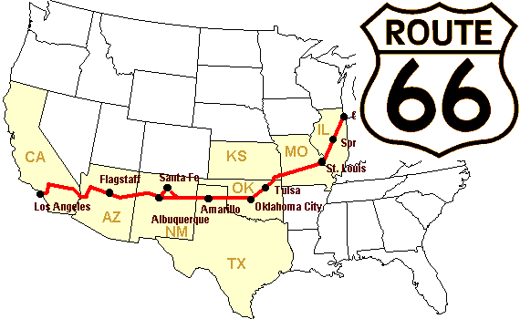
Worked example: Route 66

Let’s construct an array of distances (in miles) between cities of Route 66: Chicago, Springfield, Saint-Louis, Tulsa, Oklahoma City, Amarillo, Santa Fe, Albuquerque, Flagstaff and Los Angeles.

>>> mileposts = np.array([0, 198, 303, 736, 871, 1175, 1475, 1544,
...        1913, 2448])
>>> distance_array = np.abs(mileposts - mileposts[:, np.newaxis])
>>> distance_array
array([[   0,  198,  303,  736,  871, 1175, 1475, 1544, 1913, 2448],
       [ 198,    0,  105,  538,  673,  977, 1277, 1346, 1715, 2250],
       [ 303,  105,    0,  433,  568,  872, 1172, 1241, 1610, 2145],
       [ 736,  538,  433,    0,  135,  439,  739,  808, 1177, 1712],
       [ 871,  673,  568,  135,    0,  304,  604,  673, 1042, 1577],
       [1175,  977,  872,  439,  304,    0,  300,  369,  738, 1273],
       [1475, 1277, 1172,  739,  604,  300,    0,   69,  438,  973],
       [1544, 1346, 1241,  808,  673,  369,   69,    0,  369,  904],
       [1913, 1715, 1610, 1177, 1042,  738,  438,  369,    0,  535],
       [2448, 2250, 2145, 1712, 1577, 1273,  973,  904,  535,    0]])

Distances

Given an array of latitudes and longitudes of major European capitals calculate pairwise distances between them. Use the approximate formula:

$$D=6371.009\sqrt{(\Delta\phi)^2 + (\Delta\lambda)^2}\qquad \text{(in kilometers)},$$

where $\Delta\phi=\phi_1-\phi_2$ and $\Delta\lambda=\lambda_1-\lambda_2$ are the differences between the latitudes and longitude of two cities in radians. (Hint: To convert degrees to radians multiply them by $\pi/180$).

coords = np.array([
                  [ 23.71666667,  37.96666667], # Athens
                  [ 13.38333333,  52.51666667], # Berlin
                  [ -0.1275    ,  51.50722222], # London
                  [ -3.71666667,  40.38333333], # Madrid
                  [  2.3508    ,  48.8567    ], # Paris
                  [ 12.5       ,  41.9       ]  # Rome
                    ]) 

When you are done you can compare the results with a more precise formula:

$$D=6371.009\sqrt{(\Delta\phi)^2 + (\cos(\phi_m)\Delta\lambda)^2}$$

where $\phi_m = (\phi_1+\phi_2) / 2$ is the mean latitude.

Key Points